Ford–Fulkerson algorithm

The Ford–Fulkerson Method (named for L. R. Ford, Jr. and D. R. Fulkerson) computes the maximum flow in a flow network. It was published in 1956. The name "Ford–Fulkerson" is often also used for the Edmonds–Karp algorithm, which is a specialization of Ford–Fulkerson.

The idea behind the algorithm is very simple: As long as there is a path from the source (start node) to the sink (end node), with available capacity on all edges in the path, we send flow along one of these paths. Then we find another path, and so on. A path with available capacity is called an augmenting path.

1 Algorithm
2 Complexity
3 Integral example
4 Non-terminating example
5 Python implementation
- 5.1 Usage example
6 Notes
7 References
8 External links

Algorithm

Let $G(V,E)$ be a graph, and for each edge from $u$ to $v$ , let $c(u,v)$ be the capacity and $f(u,v)$ be the flow. We want to find the maximum flow from the source $s$ to the sink $t$ . After every step in the algorithm the following is maintained:

Capacity constraints:	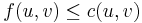$\ f(u,v) \le c(u,v)$	The flow along an edge can not exceed its capacity.
Skew symmetry:	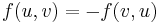$\ f(u,v) = - f(v,u)$	The net flow from $u$ to $v$ must be the opposite of the net flow from $v$ to $u$ (see example).
Flow conservation:	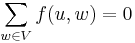$\sum_{w \in V} f(u,w) = 0$	That is, unless $u=s$ or $w=t$ . The net flow to a node is zero, except for the source, which "produces" flow, and the sink, which "consumes" flow.

This means that the flow through the network is a legal flow after each round in the algorithm. We define the residual network $G_f(V,E_f)$ to be the network with capacity 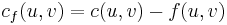$c_f(u,v) = c(u,v) - f(u,v)$ and no flow. Notice that it can happen that a flow from $v$ to $u$ is allowed in the residual network, though disallowed in the original network: if $f(u,v)>0$ and $c(v,u)=0$ then $c_f(v,u)=c(v,u)-f(v,u)=f(u,v)>0$ .

Algorithm Ford–Fulkerson

Inputs Graph $G$ with flow capacity $c$ , a source node $s$ , and a sink node $t$

Output A flow $f$ from $s$ to $t$ which is a maximum

$f(u,v) \leftarrow 0$ for all edges $(u,v)$
While there is a path from to in , such that 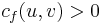for all edges :
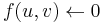
1. Find $c_f(p) = \min\{c_f(u,v)�: (u,v) \in p\}$
2. For each edge
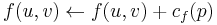  1. $f(u,v) \leftarrow f(u,v) %2B c_f(p)$ (Send flow along the path)
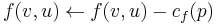  2. $f(v,u) \leftarrow f(v,u) - c_f(p)$ (The flow might be "returned" later)

The path in step 2 can be found with for example a breadth-first search or a depth-first search in $G_f(V,E_f)$ . If you use the former, the algorithm is called Edmonds–Karp.

When no more paths in step 2 can be found, $s$ will not be able to reach $t$ in the residual network. If $S$ is the set of nodes reachable by $s$ in the residual network, then the total capacity in the original network of edges from $S$ to the remainder of $V$ is on the one hand equal to the total flow we found from $s$ to $t$ , and on the other hand serves as an upper bound for all such flows. This proves that the flow we found is maximal. See also Max-flow Min-cut theorem.

Complexity

By adding the flow augmenting path to the flow already established in the graph, the maximum flow will be reached when no more flow augmenting paths can be found in the graph. However, there is no certainty that this situation will ever be reached, so the best that can be guaranteed is that the answer will be correct if the algorithm terminates. In the case that the algorithm runs forever, the flow might not even converge towards the maximum flow. However, this situation only occurs with irrational flow values. When the capacities are integers, the runtime of Ford-Fulkerson is bounded by $O(E f)$ (see big O notation), where $E$ is the number of edges in the graph and $f$ is the maximum flow in the graph. This is because each augmenting path can be found in $O(E)$ time and increases the flow by an integer amount which is at least $1$ .

A variation of the Ford–Fulkerson algorithm with guaranteed termination and a runtime independent of the maximum flow value is the Edmonds–Karp algorithm, which runs in $O(VE^2)$ time.

Integral example

The following example shows the first steps of Ford–Fulkerson in a flow network with 4 nodes, source $A$ and sink $D$ . This example shows the worst-case behaviour of the algorithm. In each step, only a flow of $1$ is sent across the network. If breadth-first-search were used instead, only two steps would be needed.

Path	Capacity	Resulting flow network
Initial flow network
$A,B,C,D$	$\min(c_f(A,B), c_f(B,C), c_f(C,D))=$ $\min(c(A,B)-f(A,B) ,c(B,C)-f(B,C), c(C,D)-f(C,D))=$ $\min(1000-0, 1-0, 1000-0)=1$
$A,C,B,D$	$\min(c_f(A,C), c_f(C,B), c_f(B,D))=$ $\min(c(A,C)-f(A,C), c(C,B)-f(C,B), c(B,D)-f(B,D))=$ $\min(1000-0, 0-(-1), 1000-0)=1$
After 1998 more steps …
Final flow network

Notice how flow is "pushed back" from $C$ to $B$ when finding the path $A,C,B,D$ .

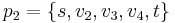
Non-terminating example

Consider the flow network shown on the right, with source $s$ , sink $t$ , capacities of edges $e_1$ , $e_2$ and $e_3$ respectively $1$ , $r=(\sqrt{5}-1)/2$ and $1$ and the capacity of all other edges some integer $M \ge 2$ . The constant $r$ was chosen so, that $r^2 = 1 - r$ . We use augmenting paths according to the following table, where 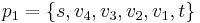$p_1 = \{ s, v_4, v_3, v_2, v_1, t \}$ , $p_2 = \{ s, v_2, v_3, v_4, t \}$ and $p_3 = \{ s, v_1, v_2, v_3, t \}$ .

Step	Augmenting path	Sent flow	Residual capacities
Step	Augmenting path	Sent flow	$e_1$	$e_2$	$e_3$
0			$r^0=1$	$r$	$1$
1	$\{ s, v_2, v_3, t \}$	$1$	$r^0$	$r^1$	$0$
2	$p_1$	$r^1$	$r^2$	$0$	$r^1$
3	$p_2$	$r^1$	$r^2$	$r^1$	$0$
4	$p_1$	$r^2$	$0$	$r^3$	$r^2$
5	$p_3$	$r^2$	$r^2$	$r^3$	$0$

Note that after step 1 as well as after step 5, the residual capacities of edges $e_1$ , $e_2$ and $e_3$ are in the form $r^n$ , $r^{n%2B1}$ and $0$ , respectively, for some $n \in \mathbb{N}$ . This means that we can use augmenting paths $p_1$ , $p_2$ , $p_1$ and $p_3$ infinitely many times and residual capacities of these edges will always be in the same form. Total flow in the network after step 5 is $1 %2B 2(r^1 %2B r^2)$ . If we continue to use augmenting paths as above, the total flow converges to 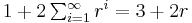$\textstyle 1 %2B 2\sum_{i=1}^\infty r^i = 3 %2B 2r$ , while the maximum flow is $2M %2B 1$ . In this case, the algorithm never terminates and the flow doesn't even converge to the maximum flow.^[1]

Python implementation

class Edge(object):
    def __init__(self, u, v, w):
        self.source = u
        self.sink = v
        self.capacity = w
    def __repr__(self):
        return "%s->%s:%s" % (self.source, self.sink, self.capacity)
 
class FlowNetwork(object):
    def __init__(self):
        self.adj = {}
        self.flow = {}
 
    def add_vertex(self, vertex):
        self.adj[vertex] = []
 
    def get_edges(self, v):
        return self.adj[v]
 
    def add_edge(self, u, v, w=0):
        if u == v:
            raise ValueError("u == v")
        edge = Edge(u,v,w)
        redge = Edge(v,u,0)
        edge.redge = redge
        redge.redge = edge
        self.adj[u].append(edge)
        self.adj[v].append(redge)
        self.flow[edge] = 0
        self.flow[redge] = 0
 
    def find_path(self, source, sink, path):
        if source == sink:
            return path
        for edge in self.get_edges(source):
            residual = edge.capacity - self.flow[edge]
            if residual > 0 and not (edge,residual) in path:
                result = self.find_path( edge.sink, sink, path + [(edge,residual)] ) 
                if result != None:
                    return result
 
    def max_flow(self, source, sink):
        path = self.find_path(source, sink, [])
        while path != None:
            flow = min(res for edge,res in path)
            for edge,res in path:
                self.flow[edge] += flow
                self.flow[edge.redge] -= flow
            path = self.find_path(source, sink, [])
        return sum(self.flow[edge] for edge in self.get_edges(source))

Usage example

For the example flow network in maximum flow problem we do the following:

g=FlowNetwork()
map(g.add_vertex, ['s','o','p','q','r','t'])
g.add_edge('s','o',3)
g.add_edge('s','p',3)
g.add_edge('o','p',2)
g.add_edge('o','q',3)
g.add_edge('p','r',2)
g.add_edge('r','t',3)
g.add_edge('q','r',4)
g.add_edge('q','t',2)
print g.max_flow('s','t')

Output: 5

Notes

^ Zwick, Uri (21 August 1995). "The smallest networks on which the Ford-Fulkerson maximum flow procedure may fail to terminate". Theoretical Computer Science 148 (1): 165–170. doi:10.1016/0304-3975(95)00022-O.

References

Cormen, Thomas H.; Leiserson, Charles E.; Rivest, Ronald L.; Stein, Clifford (2001). "Section 26.2: The Ford–Fulkerson method". Introduction to Algorithms (Second ed.). MIT Press and McGraw–Hill. pp. 651–664. ISBN 0-262-03293-7.
George T. Heineman, Gary Pollice, and Stanley Selkow (2008). "Chapter 8:Network Flow Algorithms". Algorithms in a Nutshell. Oreilly Media. pp. 226–250. ISBN 978-0-596-51624-6.
Ford, L. R.; Fulkerson, D. R. (1956). "Maximal flow through a network". Canadian Journal of Mathematics 8: 399–404.

External links

Media related to [//commons.wikimedia.org/wiki/Category:Ford%E2%80%93Fulkerson_algorithm Ford–Fulkerson algorithm] at Wikimedia Commons